User manual
Layout
Learn the toolbar, Project Explorer, main views, status bar, and the purpose of each workspace.
Tool BarTool BarTool BarTool BarThe main interface is shown in Figure 4-1.
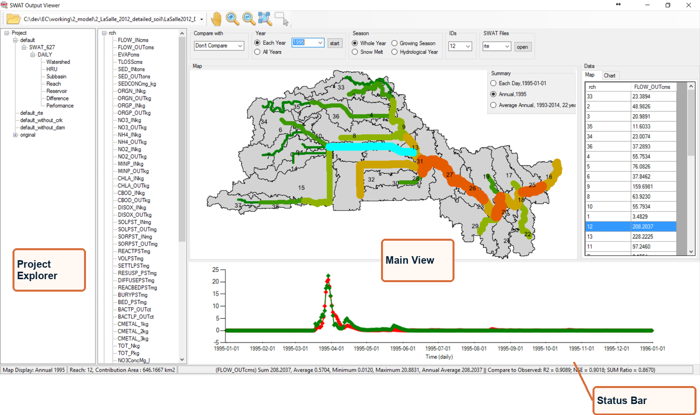
Figure 4-1. Layout of SWAT Output Viewer
The interface is comprised of four components.
Tool Bar – Function buttons to open project and select features from map;
Project Explorer – A tree view show available scenario and outputs;
Main View – Where the data is defined and displayed in graph and/or on map;
Status Bar – Information of select SWAT component and statistical information.
Tool Bar
The bool bar is located at top of the window. It’s used to open a SWAT project, explore map and select features.

Figure 4-2. Tool Bar
Once the project is opened, it will be added to the recent project list and could be selected from the drop-down list.
The Pan, Zoom in, Zoom out, Zoom Extent and Select button are applied to the map. If there is no map in current view, they will be disabled.
Project Explorer
Project Explorer is a tree structure showing all available outputs in current project. There are five levels as shown in Figure 4-3.
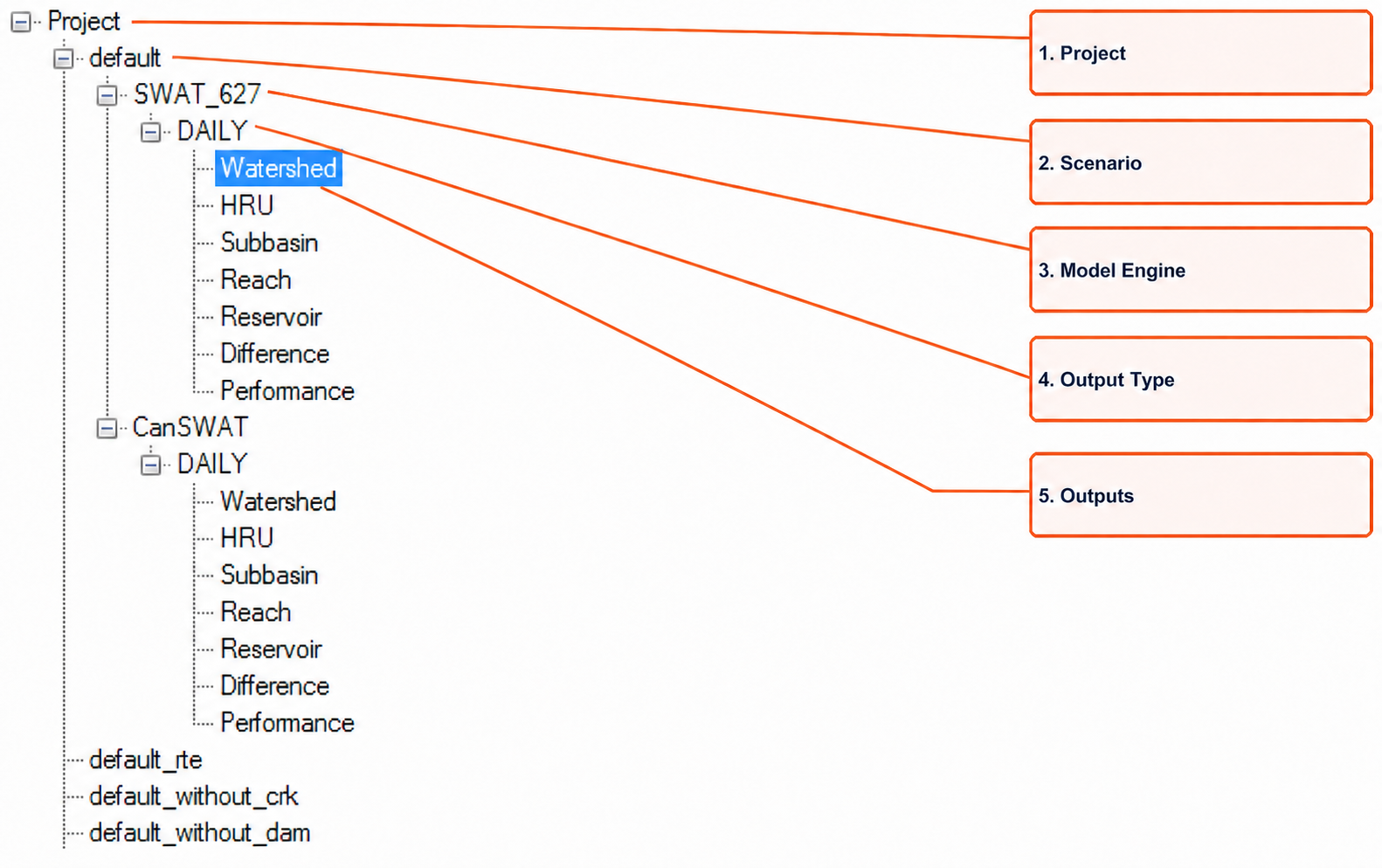
Figure 4-3. Project Explorer
The first level is Project. It’s used to set data for the whole project, i.e. the observed data.
The second level, scenario, represents a model in the Scenarios folder. The scenario is only valid when the textinout filder has all the model files.
Next is the model engine level. As different model engine could run on same model files, a scenario would have more than one output dataset.
With different output settings, same model engine may generate daily, monthly or yearly outputs. This is the fourth level.
The last the level is the Outputs level, which is used to guide through outputs of different type.
Main View
Main View is where the outputs are displayed. Different views are triggered by selecting different nodes in Project Explorer. In current version, nine types of Main View are supported. The first two views are not for outputs but necessary for importing observed data and running the model. The other seven views are for outputs of different SWAT components.
Project View – A map with all subbasins, reaches and reservoirs to allow import observed data. The observed data will be used to be shown in time series graphs besides the simulation values. It’s also used to calculate the performance statistics.
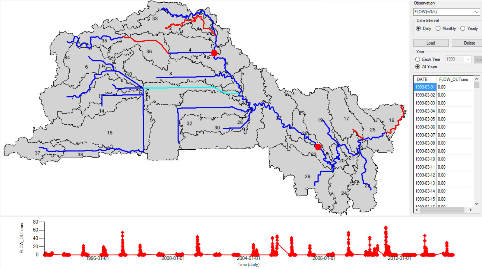
Figure 4-4. Project View
Scenario View – A view to allow run simulation, open and edit several key parameter files (file.cio, basin.bsn and fig.fig), open the model folder and copy the txtinout folder to SWAT_CUP backup folder. If working on a modified version of SWAT, you could also select different version of SWAT to run.
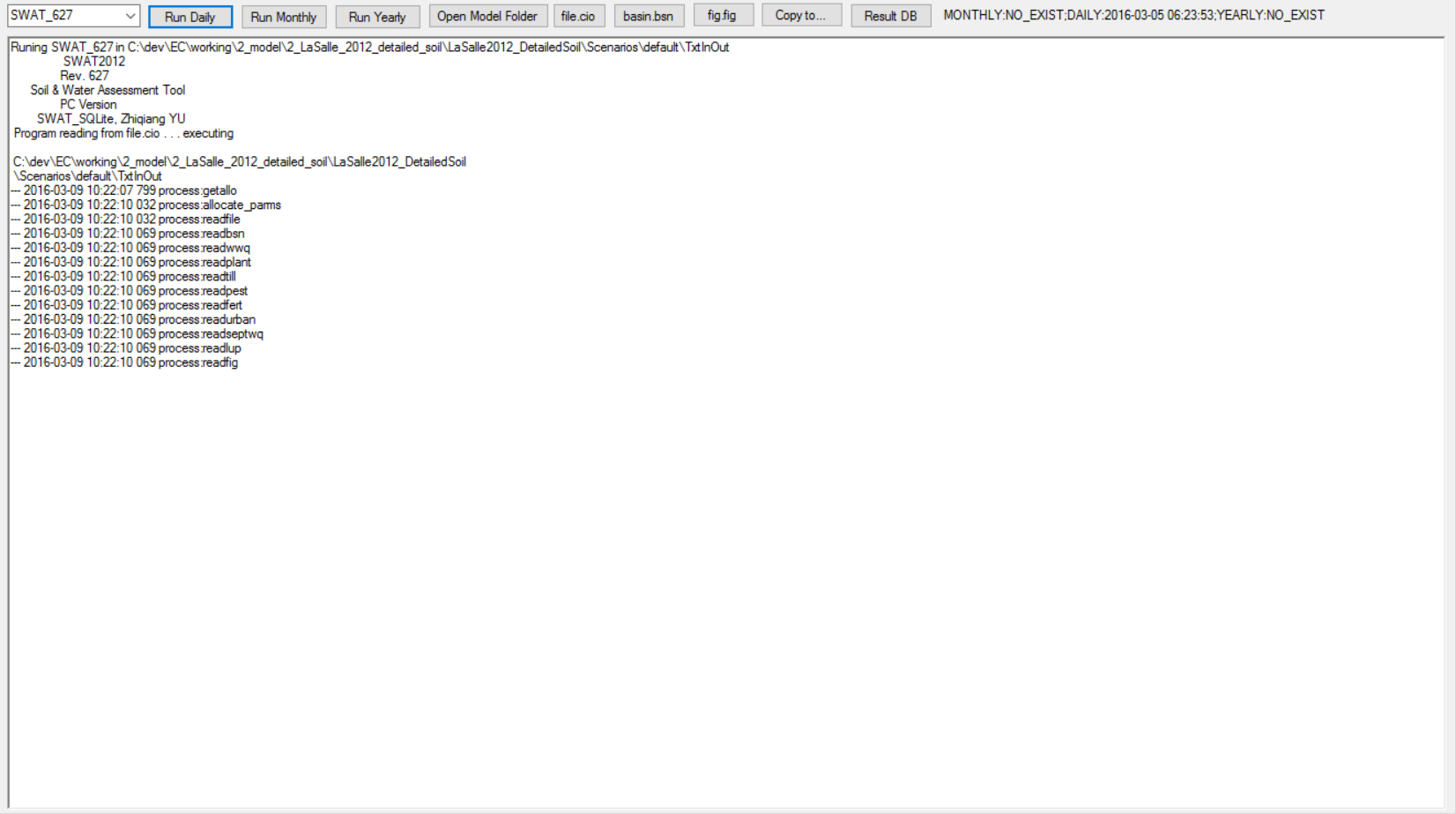
Figure 4-5. Scenario View
Watershed View – Outputs of watershed level which is corresponding to the outputs in output.std.
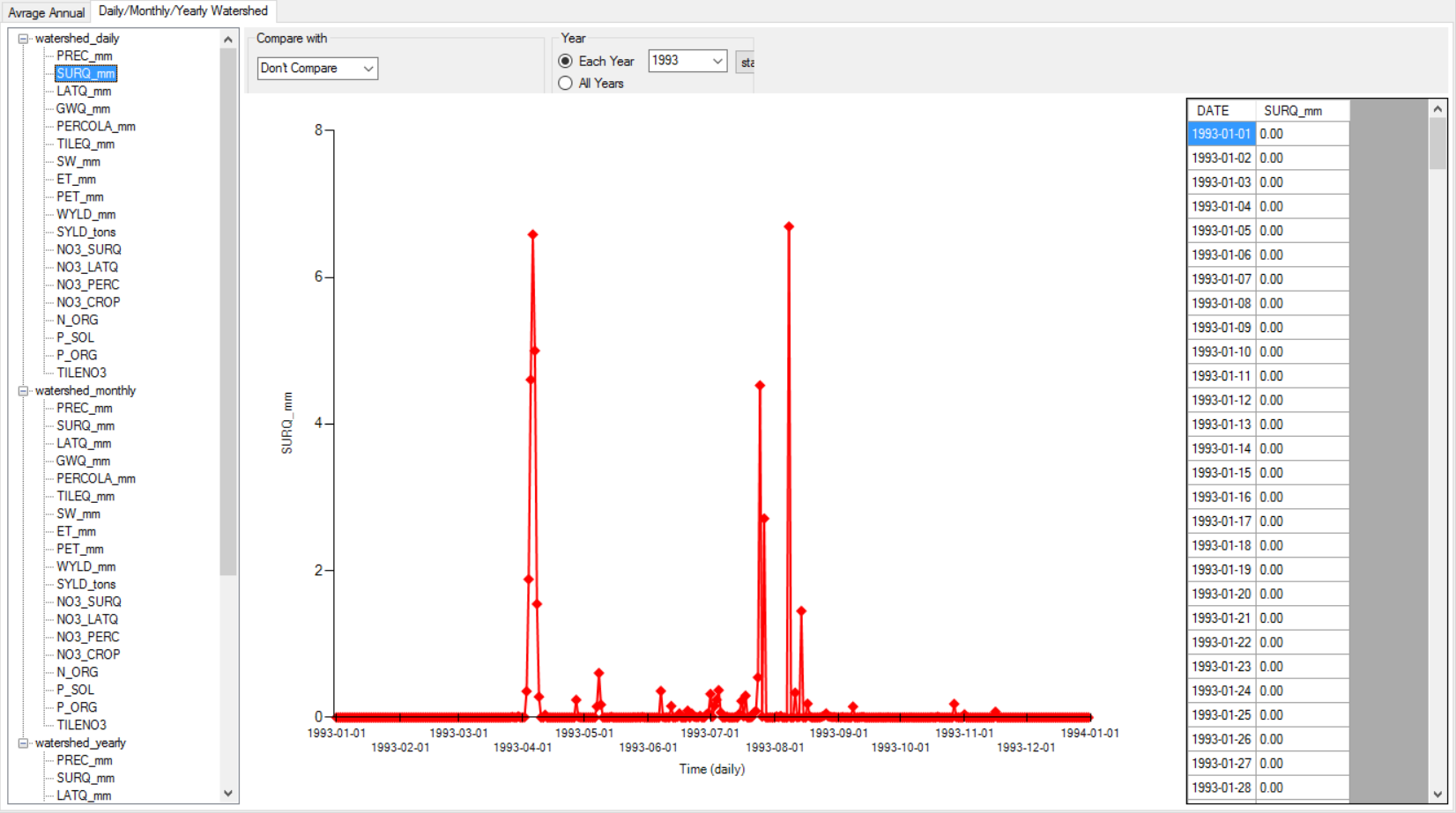
Figure 4-6. Scenario View
HRU View – HRU outputs (mainly output.hru) with map, table and graph. As HRU don’t have spatial locations, the subbasin layer is used to help locate the HRU.
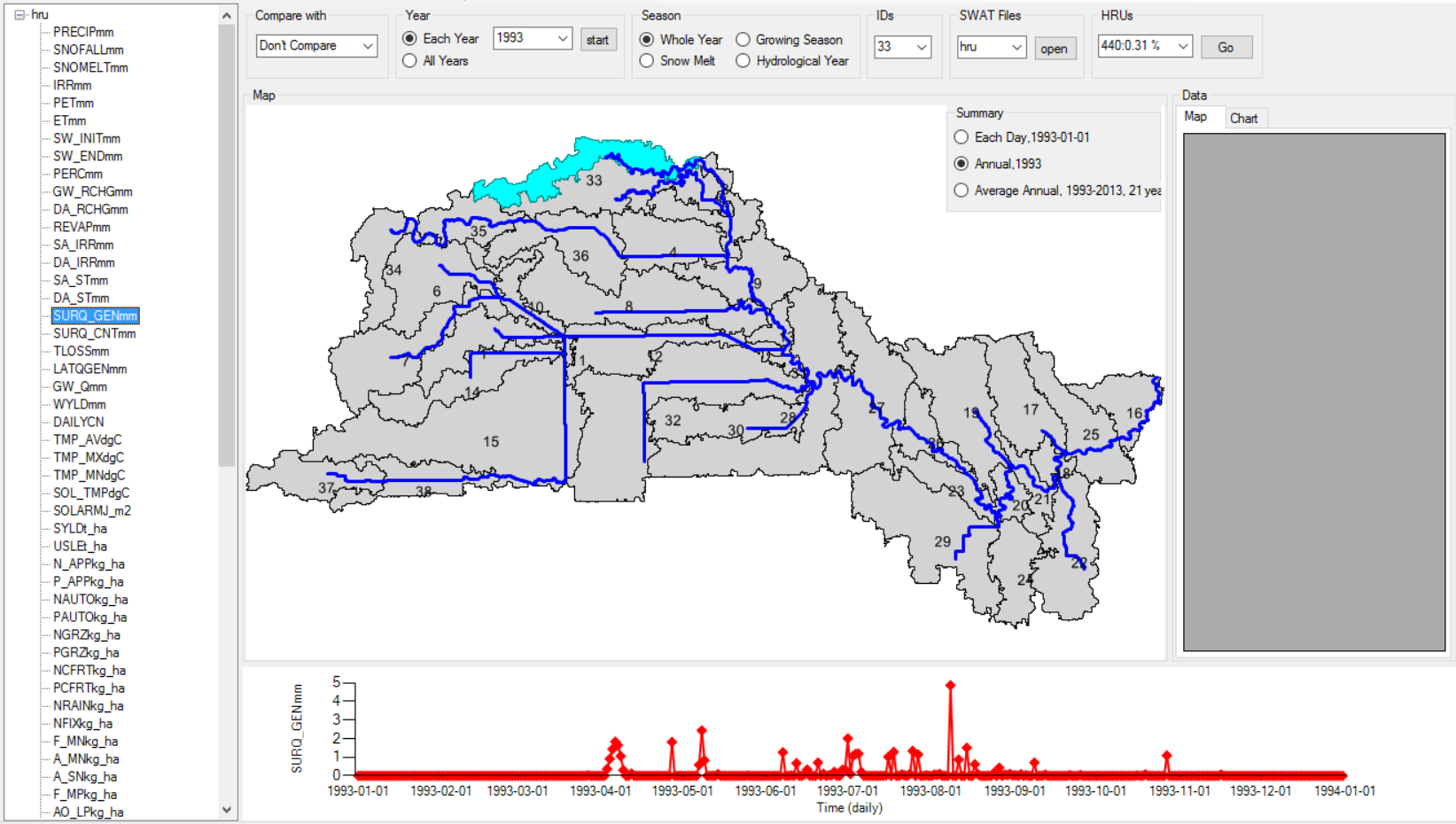
Figure 4-7. HRU View
Subbasin View – Time series graph and thematic map for subbasin outputs (output.sub)
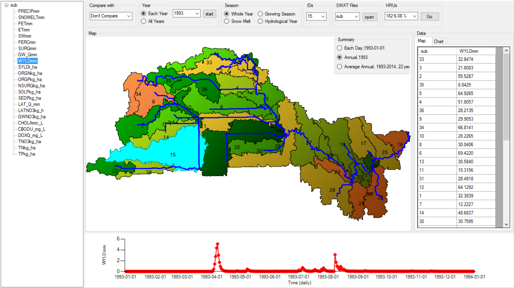
Figure 4-8. Subbasin View
Reach View – Time series graph and thematic map for reach outputs (output.rch, output.sed)
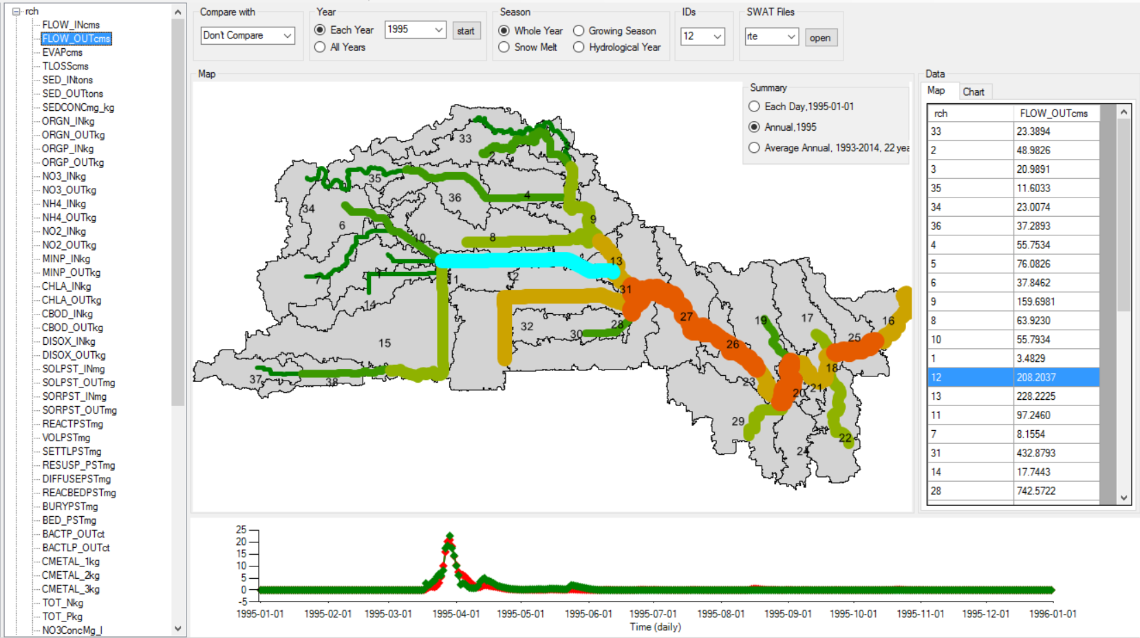
Figure 4-9. Reach View
Reservoir View – Time series graph for reservoir outputs (output.rsv)
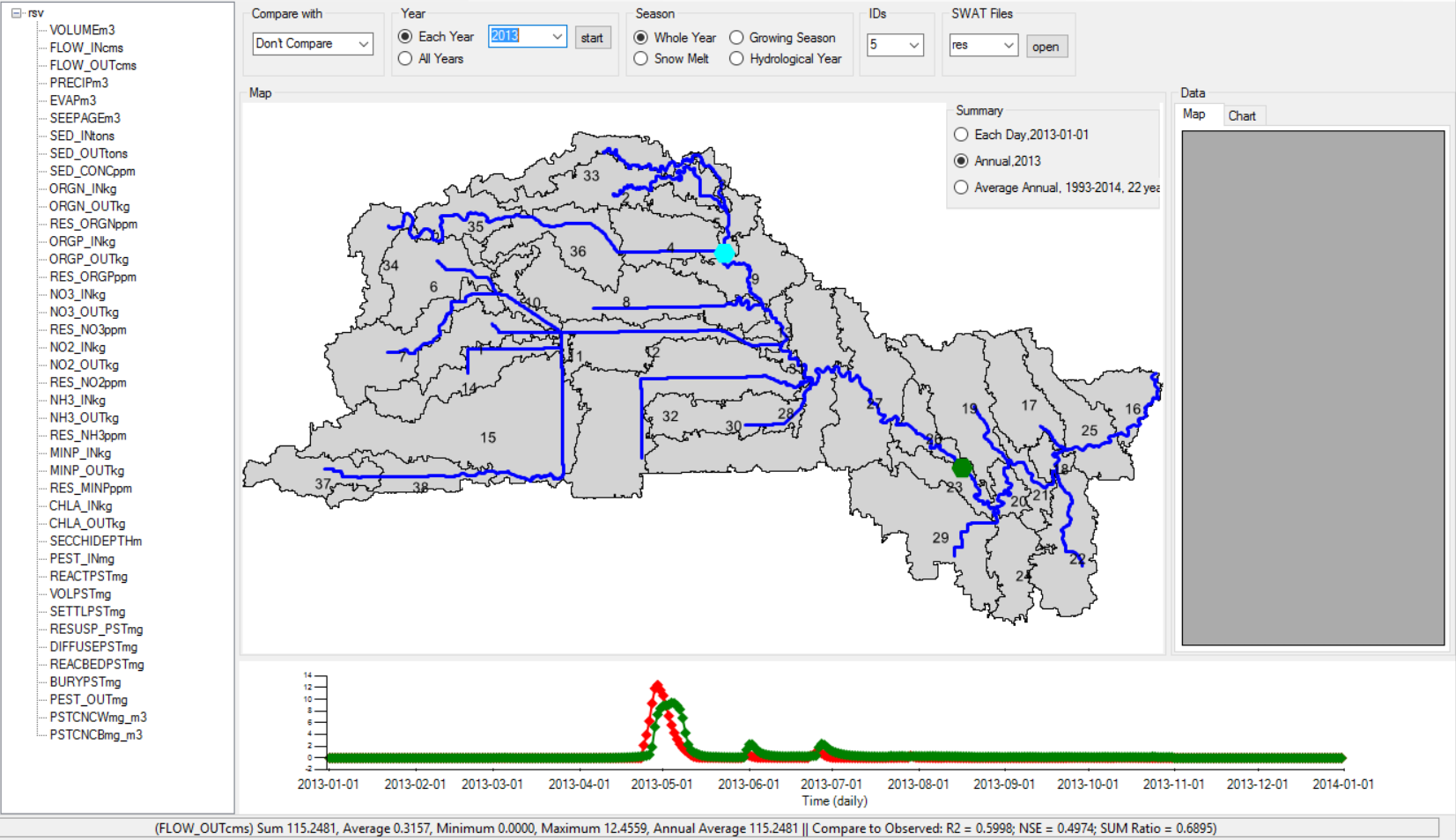
Figure 4-10. Reservoir View
Difference View – Compare outputs of same components from different model or scenarios. R2 is given as the indicator how different they are.
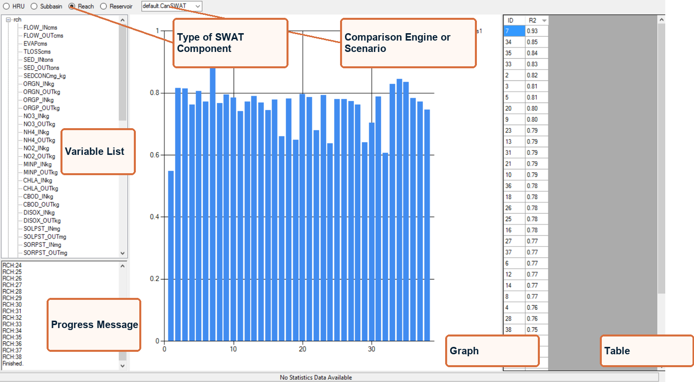
Figure 4-11. Difference View
Performance View – Show various performance statistic (NSE, bias, RMSE, etc.)
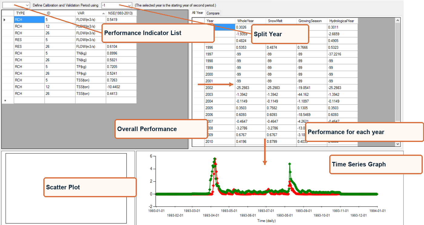
Figure 4-12. Performance View
Status Bar
Status bar is located at bottom of the interface. It shows there type of information.
The year selected as the time range of outputs;
The basic information of selected SWAT component;
The statistics for current time series data. If only one time series is available, sum, average, min and max is displayed. If more than one time series data (observed and/or comparison) is available, R2 and NSE is also displayed.