User manual
Viewing Outputs
Explore watershed, HRU, subbasin, reach, and reservoir results using maps, tables, graphs, comparisons, and exports.
Views for SWAT Outputs
In SWAT Output Viewer, SWAT outputs are displayed in several views based on the type of model component or level it belongs to. Table 7-1 lists all the SWAT output files and the view to display it in SWAT Output Viewer. All the outputs are categorized into five groups (watershed, HRU, subbasin, reach and reservoir). Each group has a corresponding view in SWAT Output Viewer for data display.
Table 7-1. SWAT Output Files and Corresponding Views in SWAT Output Viewer
| Index | SWAT Output File | Description | View in SWAT Output Viewer |
|---|---|---|---|
| 1 | output.std | Standard output file | Watershed |
| 2 | output.hru | HRU output file | HRU |
| 3 | output.sub | Subbasin output file | Subbasin |
| 4 | output.rch | Main channel output file | Reach |
| 5 | output.rsv | Reservoir output file | Reservoir |
| 6 | output.wtr | HRU impoundment output file | HRU |
| 7 | output.pot | Pothole output file | HRU |
| 8 | output.mgt | Management output file | HRU |
| 9 | output.snu | Soil nutrient output file | HRU |
| 10 | output.swr | Soil water output file | HRU |
| 11 | output.sed | Sediment loads output file | Reach |
Layout of Views
Except for watershed view, all other four views are using the same layout as shown in Figure 7-1. The view is comprised of five information panels: 1) Variable List, 2) Control Bar, 3) Map, 4) Table and 5) Graph.
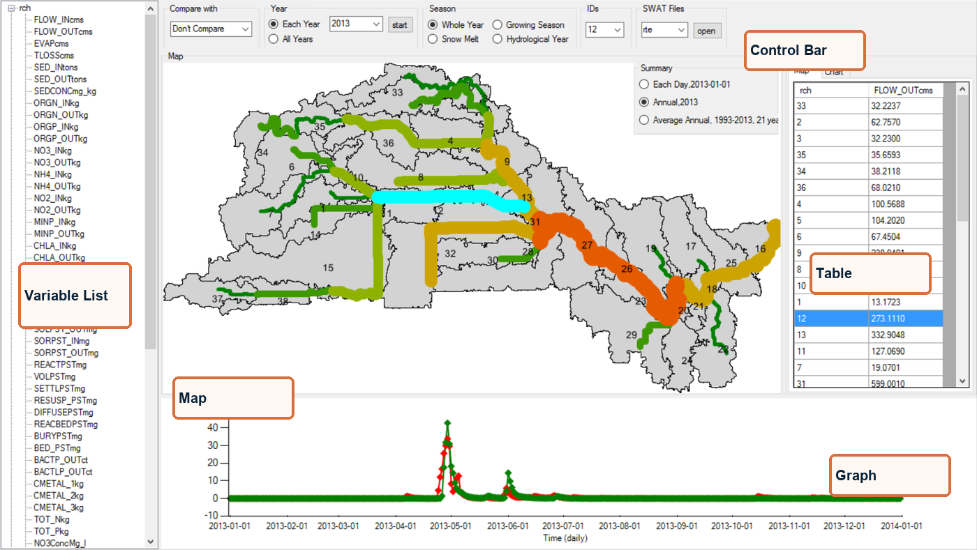
Figure 7-1. Layout of Reach View
Variable List
Variable List is used to define which output variable will be displayed. It lists all available output variables in a tree structure. The first level is the extension of the SWAT output file, such as rch and sub. All output variables in that file are list in the second level. From Table 7-1, HRU view has the ability to show outputs from six output files. So it may have six first level nodes. Reach view may have two (rch and sed). Subbasin and reservoir view would only have one.
Control Bar
Control Bar controls how the data is displayed.
Defining Time Range
The time period of time series data could be defined with Year and Season section. For a daily model running for several years, generally it’s a good idea to see the outputs year by year. This could be done by select the Each Year option and select the year. It’s also possible to go through all years by click the start button.
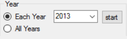
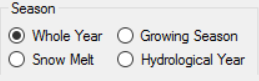
Figure 7-2. Year and Season Control in Control Bar
Season is a pre-defined time period in one year. It help to see the model behavior in certain time period. Four seasons are available in current version: 1) Whole Year (Jan – Dec), 2) Growing Season (May - Oct), 3) Snow Melt (Mar – May) and 4) Hydrological Year (Oct – Sep). Once one season is selected, only data in that time range will be displayed in graph. An example is shown in Figure 7-3, where year is 2013 and snow melt is selected.

Figure 7-3. Graph for Reach Flow in 2013 Snow Melt Period
Selecting SWAT Component
The IDs list could be used select the model component for time series data display. The ID of all available SWAT components are list in the list. And this list is synced with map selection, i.e. the selection in IDs list and the selection on map will change each other. Although it’s generally easier to make the selection on map, it’s easier to use the IDs list when you don’t know the location of a specific component.

Figure 7-4. IDs List in Control Bar
Once a SWAT component is selected, its key information is displayed in the status bar as shown in Figure 7-5. The main information displayed is area (HRU and subbasin) or drainage area (reach).



Figure 7-5. SWAT Component Inform in Status Bar
Viewing and Editing Model Files
The SWAT Files section gives the opportunity to open model files for selected model component. As there may be more than one model files, a list is given to specify the extension of the file. This could be used to make sure changes to parameters are applied. Minor changes could be also made here.
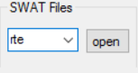
Figure 7-6. SWAT Files in Control Bar
Defining Comparison Outputs
The Compare with section allows to add comparison dataset to the time series graph. The available comparison dataset includes 1) outputs from different scenarios but with same model engine and 2) outputs generated with different model engine on same scenario. It could be used to find the different between these two datasets.
As shown in Figure 7-7, the available outputs is shown in the drop list if there are some available. To distinguish them, they are named with the scenario name and model engine name.
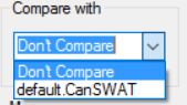
Figure 7-7. Compare with Section in Control Bar
Once the comparison outputs are selected, its data would be displayed in graph along with the original outputs as shown in Figure 7-8. Notice that the original outputs are in red and the comparison outputs are in blue. With this selection, the statistic between these two time series data would also be calculated and shown in status bar as shown in Figure 7-9, where SUM Ratio is the ratio of summation of data points in original datasets to the summation of data point in comparison datasets. In the given example, the original dataset is only 10% of the comparison dataset.
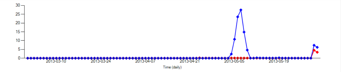
Figure 7-8. Graph Showing Time Series Data with Comparison Dataset

Figure 7-9. Statistics for Original and Comparison Dataset
For SWAT components with observed data, the comparison outputs would be displayed along with the original outputs and the observed datasets which are in green as shown in Figure 7-10. This would help identify which outputs are more close to observed data.

Figure 7-10. Graph Showing Time Series Data with Comparison and Observed Dataset
Map
Map is used to 1) select SWAT model components and 2) show the spatial distribution of selected variable in selected time range with different symbols.
Data Source
The shapefiles located at Watershed\Shapes folder are utilized as the data source for the map display. They are generated automatically in the model creation process. If they are deleted for some reason, the map couldn’t display properly.
The subbasin and reach layer is available from the shapefiles. But reservoir layer is not there. To display reservoir layer, it’s required to generate a shapefile with name monitoring_points2.shp from the MonitoringPoint feature class in project database.
Selecting Model Component on Map
Model component could be select on map (except for HRU). To select a SWAT component, click where it’s located on the map. If the selection is made successfully, the selected feature will be highlighted. To make selection precisely, only the corresponding layer is selectable, e.g. only subbasin layer is selectable in subbasin view.
As described in Selecting SWAT Component in Control Bar, the selection made on map is synced with selection made with IDs list.
Thematic Map
A thematic map is automatically generated with data from selected variable of selected subbasin and reach. With different symbols, the thematic map shows the spatial distribution of select variable, which would help identify 1) potential issues in current model and 2) key locations for targeting BMPs.
In subbasin view, the subbasins are rendered from green to red for values from low to high as the one shown in Figure 7-11.
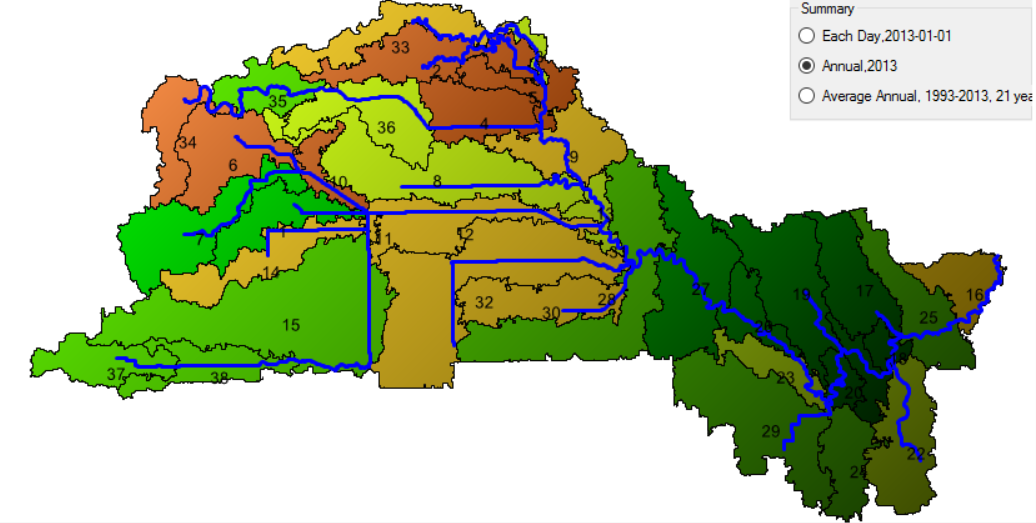
Figure 7-11. Subbasin Thematic Map for Water Yield in 2013
In reach view, reaches are drawn with different color and thickness to show how the selected variable change in the reach network.
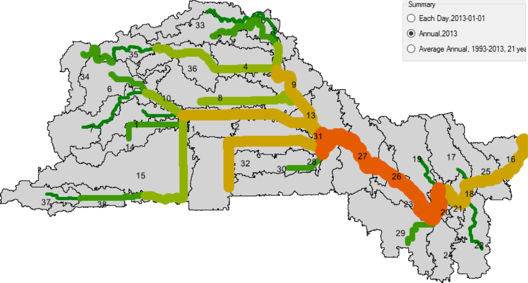
Figure 7-12. Reach Thematic Map for Flow in 2013
The thematic map supports three types of data: 1) Each day, 2) Annual and 3) Average Annual, which could be selected with the Summary control panel (Figure 7-13) located at right top corner of the map. They define how the data is summarized and then displayed on map.
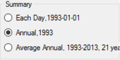
Figure 7-13. Thematic Map Data Summary Control Panel
Each day option renders the map with the data of selected day. The day could be selected from the Chart Table on right.
Annual option summarized the data for given year first and then displays on map. For loads, summation is used. For concentration, average is used. This is the default option.
Average Annual option calculates the average annual value for all available years and the displays on map.
The dataset for the thematic map could be checked out in Map Table (Figure 7-14) located at right of the map, where the data could be sorted by double-clicking the column title.
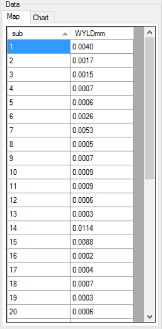
Figure 7-14. Thematic Map Data Table
The data could also be imported by selecting Export current results to CSV menu on the map.
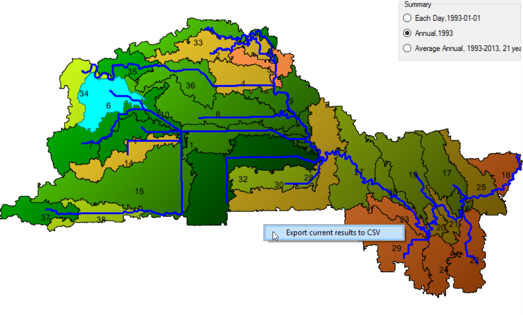
Figure 7-15. Export Current Results to CSV Menu for Thematic Map
Table
Table section show the time series data and the thematic map data in table. It has two tabs as shown in Figure 7-14. The Map tab shows the thematic map data and the Chart tab is for time series data shown in graph. Note that the Chart tab is empty in current version.
Graph
Graph shows the time series data in a graph as shown in Figure 7-16.

Figure 7-16. Time Series Graph
When observed data is available for selected SWAT component, the observed data (green) is also shown in the same graph (Figure 7-17). The observed data needs to be imported in project view. Once it’s imported, it will be automatically added to the graph.
Figure 7-17. Time Series Graph with Observed Data
When comparison outputs are selected, the time series from comparison outputs are also added to the graph in blue (Figure 7-18).
Figure 7-18. Time Series Graph with Observed Data and Comparison Outputs
The time series datasets could be downloaded by selecting Export current results to CSV menu. The exported file is saved in exports folder (in installation folder).

Figure 7-19. Export Menu in Time Series Graph
Steps to View Outputs
Time Series Data
To view time series data, follow following steps.
Select the right node in Project Explorer, e.g. select Reach for reach outputs and Subbasin for subbasin outputs.
Select the right variable in Variable List. The name of variables is similar to the column name used in SWAT output files. If one is not there, check file.cio to make sure that variable is not ignored. By default, HRU outputs are not generated.
Select the SWAT component from IDs list or on map.
Change the time range of the time series data by changing year and season.
If available, select comparison outputs for comparison.
Thematic Map
To view thematic map, go with following steps.
Select type of data and variable in Project Explorer and Variable List same as step 1 and 2 in viewing time series data.
Change year for data of that year.
Change the option for summary method to switch the data between different thematic maps.
Viewing Watershed-level Summaries
There are two tabs available in Watershed View. The Average Annual gives the average annual for the whole watershed.
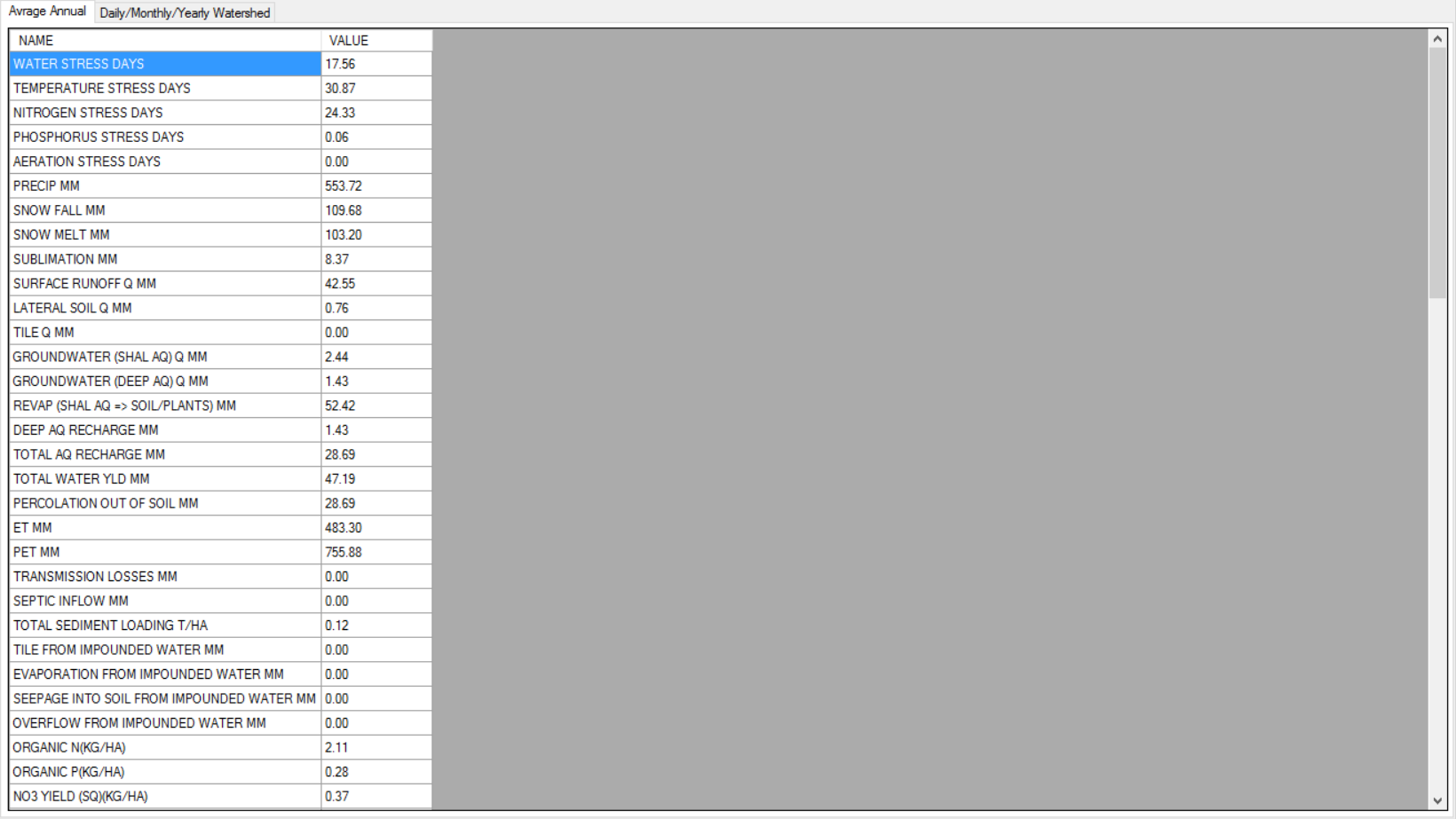
Figure 7-20. Average Annual Outputs in Watershed View
The Daily/Monthly/Yearly Watershed gives more detailed data in daily, monthly and yearly. Select the variable in the tree view on the left, the data will be shown in graph and table. For daily and monthly data, it’s also possible to view the data year by year by choosing the Each Year option and selecting the year in the drop down list.
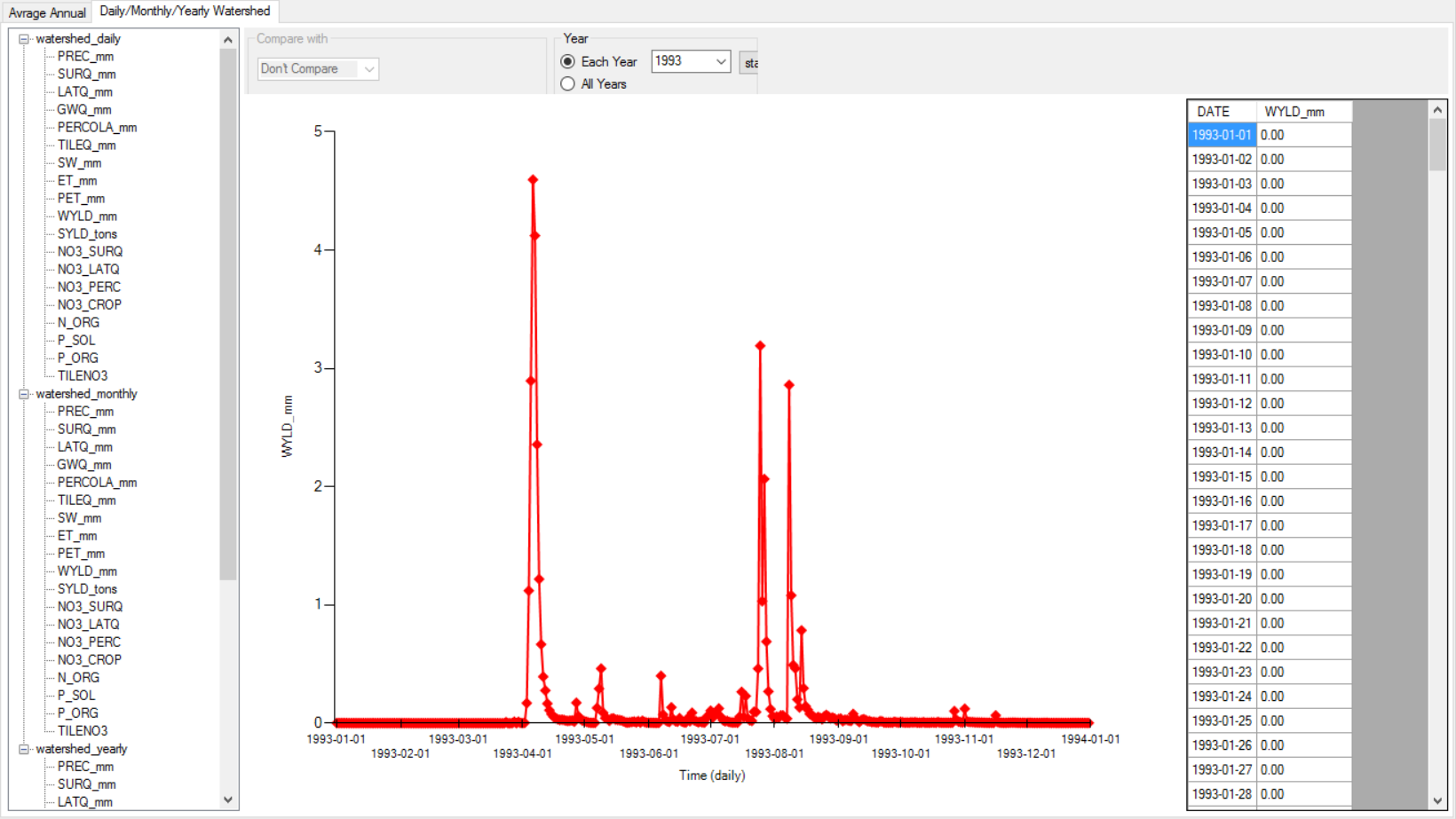
Figure 7-21. Daily, Monthly and Yearly Outputs in Watershed View
While the data is shown in graph and tables, some of the statistic information is also shown in the status bar.

Figure 7-22. Time Series Statistics for Watershed View